Machine Learning Specialization Notes

Soulter

2026-07-23

技术

模型评估

分为训练集、测试集和验证集。测试集用于评估模型最终的泛化程度。验证集主要为了调参。
选取测试集的方法一般有：留出法、交叉验证法、自助法
模型评估的一些重要量：Precision/Recall、AUC；TPR/FPR、ROC；代价加权的错误率（不单单是错误数量）。

线性模型

目标：让拟合后的函数对原始样本点在x相同时的欧氏距离总和最小
最小二乘法、极大似然估计
一元线性回归、多元线性回归。
可以进行非线性转化，即y’ = 一个可微连续函数。本质上是代换，sigmoid 就是一个典型例子，可以用于处理二分类问题。
多分类问题有OvO、OvR、MvM等。
类别不平衡时，可以采用过采样（增加正例，如插值）、欠采样（减少反例，如将多的反例丢给不同的学习器，每一个学习器正反例近似）、阈值移动
多分类学习不是多标记学习。

神经网络

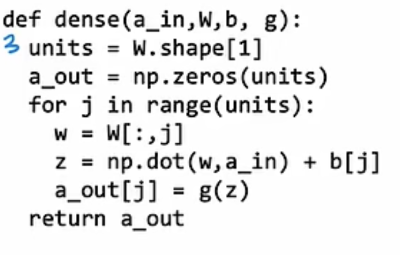
For some neural network that make up with Dense layers, we constantly use sigmoid as activation function. A hidden layer usually contains many units, a unit use the output of its previous layer as input.

$a_2^{[1]}=g(\vec{w_2^{[1]}}\cdot\vec{a^{[0]}}+b_2^{[1]})$

$a_2^{[1]}$ means the output of the second unit in the first hidden layer.

Basic

A simple training case with tensorflow：

import tensorflow as tf
from tensorflow.keras import Sequential
from tensorflow.keras.layers import Dense
from tensorflow.keras.losses import BinaryCrossEntropy

model = Sequential([
    Dense(units=25, activation='sigmoid'),
    Dense(units=15, activation='sigmoid'),
    Dense(units=1, activation='sigmoid'),
])

model.compile(loss=BinaryCrossEntropy())
model.fit(X, y, epochs=10000)

Actication function

such as sigmoid, linear…

here z means $\vec{w}\cdot\vec{x}+b$

Sigmoid

$g_{w,b}(z) = \frac{1}{1 + e^{-z}}$

Linear

no vatication function. If our network doesn’t contains activation function, so it’s a simple multiplex of matrix. 这只是线性变换。但是我们需要引入非线性的部分来让他拟合任何函数

$g_{w,b}(z)=z$

ReLU

$g_{w,b}(z) =max(0, z)$

Softmax

How to choose

For the output layer

sigmoid: binary classfication, multi lable classfication
linear: regression that y has +/-
ReLU: regression that y only has +
softmax: multi class classfication

For the hidden layers:

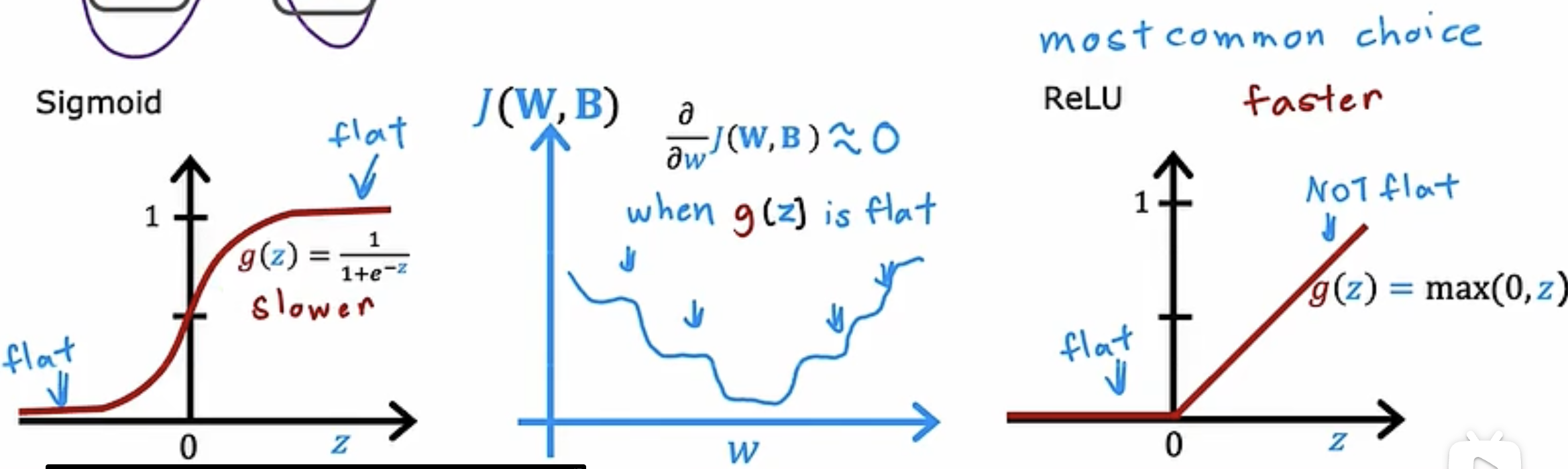
Currently, we most use ReLU than sigmod.

speed. sigmoid requires taking an exponentiation and then a inverse
regression descend speed. sigmoid has two flat place

Cost function 代价函数

the cost function sum the whole losses in the training set.

$J(\mathbf{W,B})=\frac{1}{m}\sum_{i=1}^{m}L(f(\vec{x}^{(i)}),y^{(i)})$

we should minimize the cost!

For Linear Regression, we use Mean Squared Error as cost function.

$J(\mathbf{W,B})=\frac{1}{2m}\sum_{i=1}^{m}(f(\vec{x}^{(i)})-y^{(i)})^2$

For Logistic Regression, we use Binary Cross Entropy as cost function.

$J(\mathbf{W,B})=-\frac{1}{m}\sum_{i=1}^{m}y^{(i)}log(f(\vec{x}^{(i)}))+(1-y^{(i)})log(1-f(\vec{x}^{(i)}))$

Regularization 正则化

We can add a regularization term to the cost function to prevent overfitting.

$J(\mathbf{W,B})=\frac{1}{m}\sum_{i=1}^{m}L(f(\vec{x}^{(i)}),y^{(i)})+\frac{\lambda}{2m}\sum_{l=1}^{L}||\mathbf{W}^{[l]}||^2$

$\lambda$ : regularization parameter(hyperparameter)

Some loss functions

BinaryCrossEntropy

AKA logistic loss

$L(f(\vec{x}),y)=-ylog(f(\vec{x}))-(1-y)log(1-f(\vec{x}))$

MeanSquaredError

…

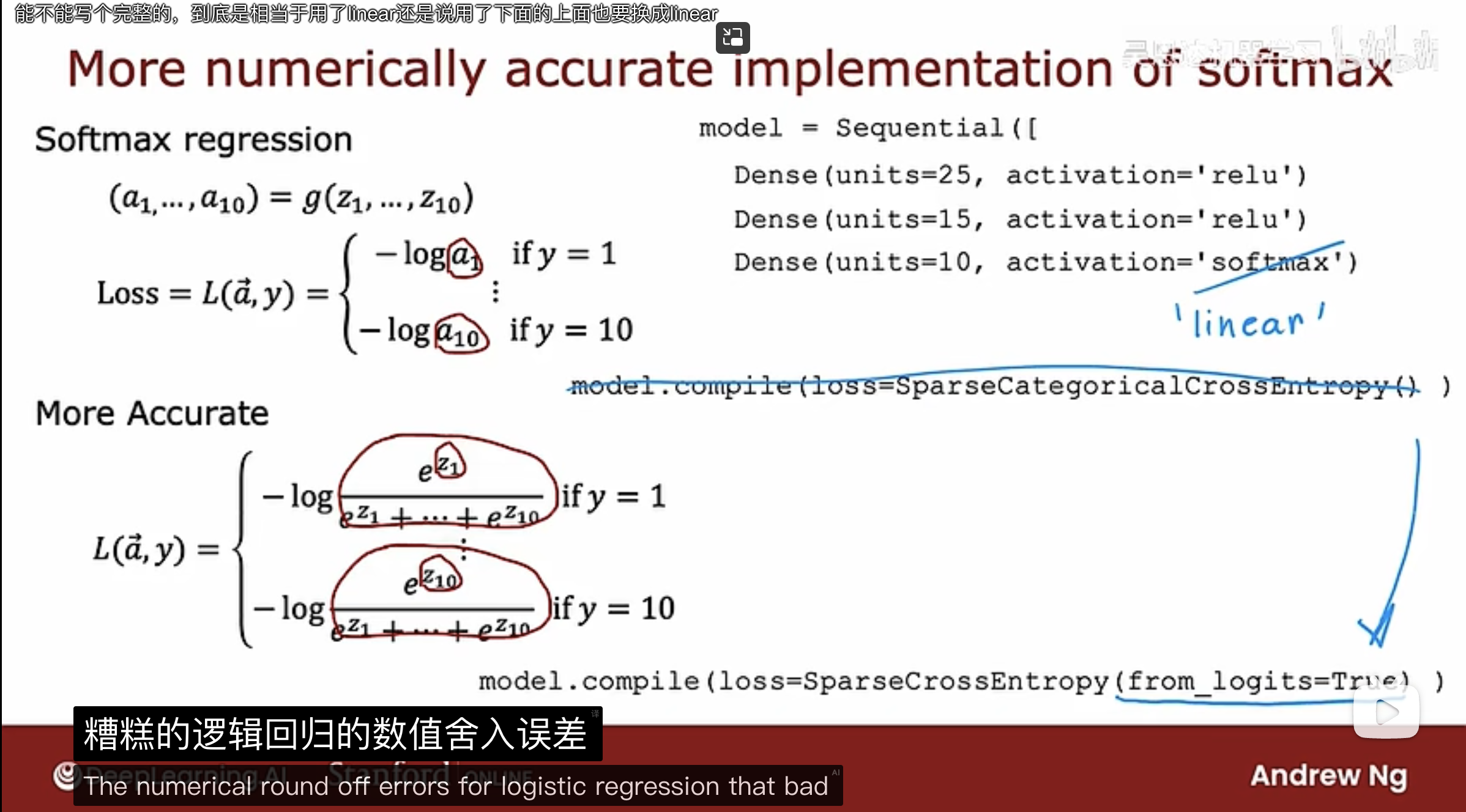
SparseCategoricalCrossEntropy

more accurate training effect:

surely, the result we got from the output layer is z1…z10 but not a1…a10, so, when we want to use it to predict new datas, we should call
1
2
logits = model(X) # X is the inputs we want to predict.
f_x = tf.nn.softmax(logits)

Gradient Descent

Recall the gradient descent algorithm utilizes the gradient calculation:

\begin{align*} &\text{repeat until convergence:} \; \lbrace \\ & \; \; \;w_j = w_j - \alpha \frac{\partial J(\mathbf{w},b)}{\partial w_j} \tag{1} \; & \text{for j := 0..n-1} \\ & \; \; \; \; \;b = b - \alpha \frac{\partial J(\mathbf{w},b)}{\partial b} \\ &\rbrace \end{align*}

Where each iteration performs simultaneous updates on $w_j$ for all $j$ , where

\begin{align*} \frac{\partial J(\mathbf{w},b)}{\partial w_j} &= \frac{1}{m} \sum\limits_{i = 0}^{m-1} (f_{\mathbf{w},b}(\mathbf{x}^{(i)}) - y^{(i)})x_{j}^{(i)} \tag{2} \\ \frac{\partial J(\mathbf{w},b)}{\partial b} &= \frac{1}{m} \sum\limits_{i = 0}^{m-1} (f_{\mathbf{w},b}(\mathbf{x}^{(i)}) - y^{(i)}) \tag{3} \end{align*}

m is the number of training examples in the data set
$f_{\mathbf{w},b}(x^{(i)})$ is the model’s prediction, while $y^{(i)}$ is the target
For a logistic regression model
$z = \mathbf{w} \cdot \mathbf{x} + b$
$f_{\mathbf{w},b}(x) = g(z)$
where $g(z)$ is the sigmoid function:
$g(z) = \frac{1}{1+e^{-z}}$

Some ways to optimize and debug training

Adam algorithm: auto learning rate

1	model.compile(optimizer=tf.keras.optimizers.Adam(learning_rate=1e-3), loss=xxx)

Fine tune params: $\lambda$ (regularization), $\alpha$ (learning rate), epoch, layers
More training sets(可以对同一个数据集进行一些变换，比如旋转、翻转、缩放等等)
More features, adding polynomial(多项式) features(x, x^2, x1x2, etc)
Early stopping（当验证集上的误差不再下降的时候，停止训练。可以防止过拟合）

Feature scaling

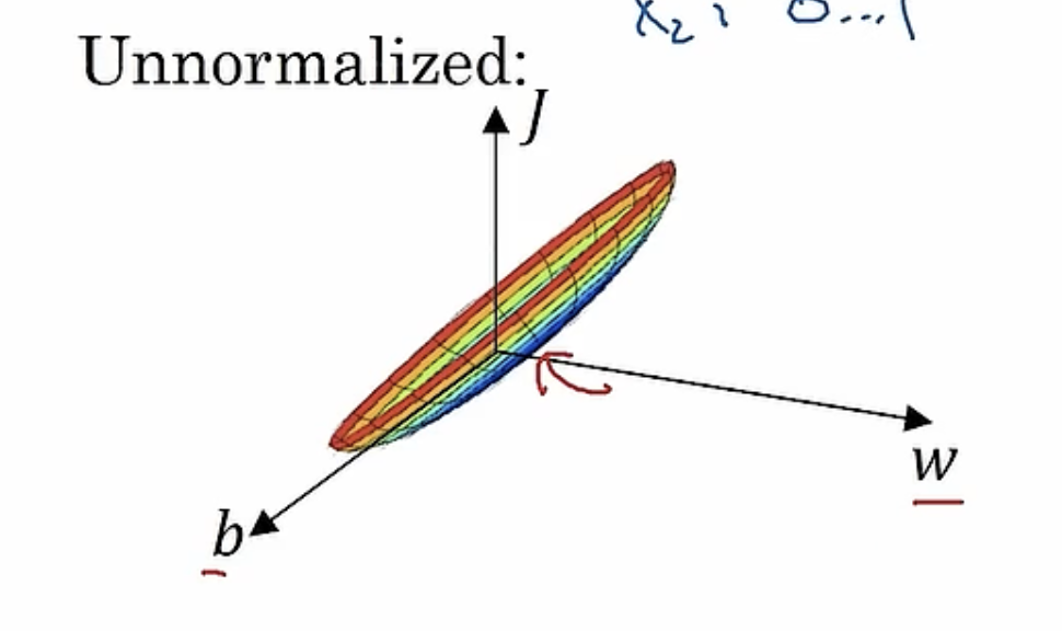
Feature scaling is a method used to standardize the range of independent variables or features of data. In data processing, it is also known as data normalization and is generally performed during the data preprocessing step.

归一化的目的是为了消除特征之间的量纲影响，使得不同特征之间具有可比性。如果不进行归一化，那么在梯度下降的过程中，不同特征的梯度差异会很大，导致收敛速度慢。

normalization

mean normalization
standardization
z-score normalization

特征工程

有时候我们需要对特征进行一些处理，比如对特征进行组合、转换、删除。这样可以让模型更好地拟合数据。

Evaluating a model

we use test set.

for the classification problem, the $J_{test}(\vec{w},b)$ is the fraction of the test set that has been misclassified.

Select a model

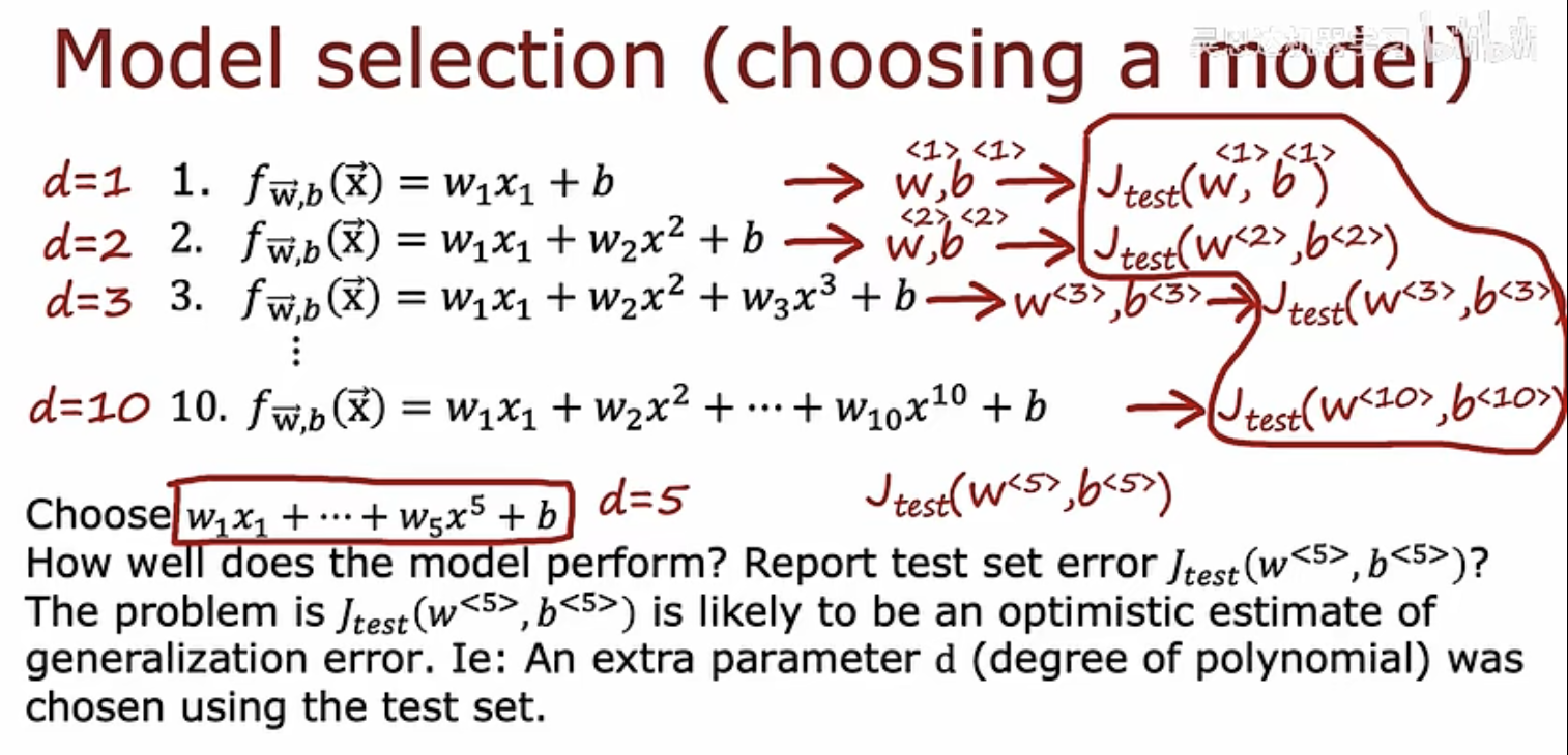
why we need to divide data to training set, dev set and test set?
dev set (a.k.a validation set) is used to fine tune the super param. 当我们从训练集合训练得到初步结果的时候，我们需要根据在验证集上的结果通过调节超参数去进一步地优化这个模型，this behavior let the model tend to “fit” the validation, 只不过不是梯度下降层面的，是手动层面的。因此，我们需要一个完全纯净的数据集去进行最后的效果验证。

Bias / variance

underfit: Jtrain and Jcv is high (high bias)
overfit: Jtrain is low but Jcv is high (high variance)

we also can optimize model via changing lambda.

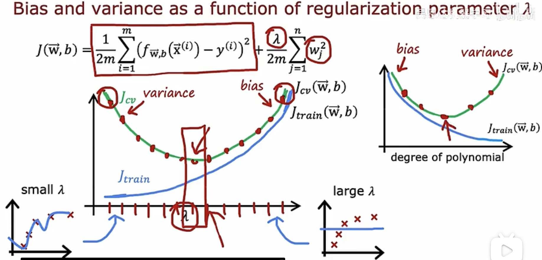
we can determine a baseline performance, so we can evaluate the effect of the model we trained. the baseline can be human’s accuracy toward this problem(such as audio2text)

Learning curves

Generally speaking, training error increases with the increase of training set size, while cross validation error decreases with the increase of training set size. This also illustrate that if a learning algorithm suffers from high bias(or data set is bad), getting more training data will not help much. For example, we use a linear funciton to fit a nonlinear data. If a learning algorithm suffers from high variance, getting more training data is likely to help.

getting more training data can reduce the gap between Jcv and Jtrain

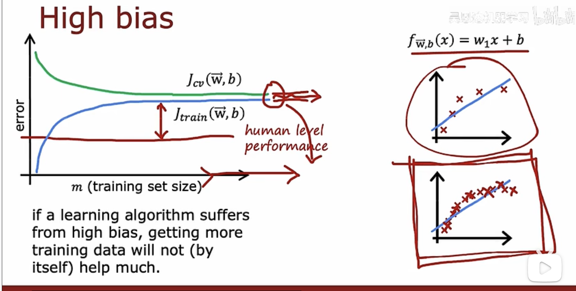
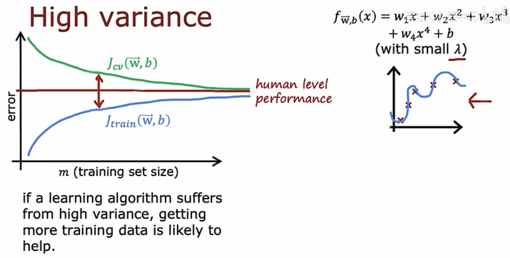
a bias variance analysis can tell you 你是否应该在某些特征上花更多的力气去收集更多的数据，因为有些特征可能没有那么大的帮助

Data augmentation

you can introduce some ‘noise’ for a data to let the model you training more powerful.

Color shift, PCA color augmentation
Ramdom crop
Rotation
Flipping

Transfer learning

fine tuning some params from a supervised pretraining model can let you get your model you want faster.

option1: only train output layers parameters.

option2: train all parameters.

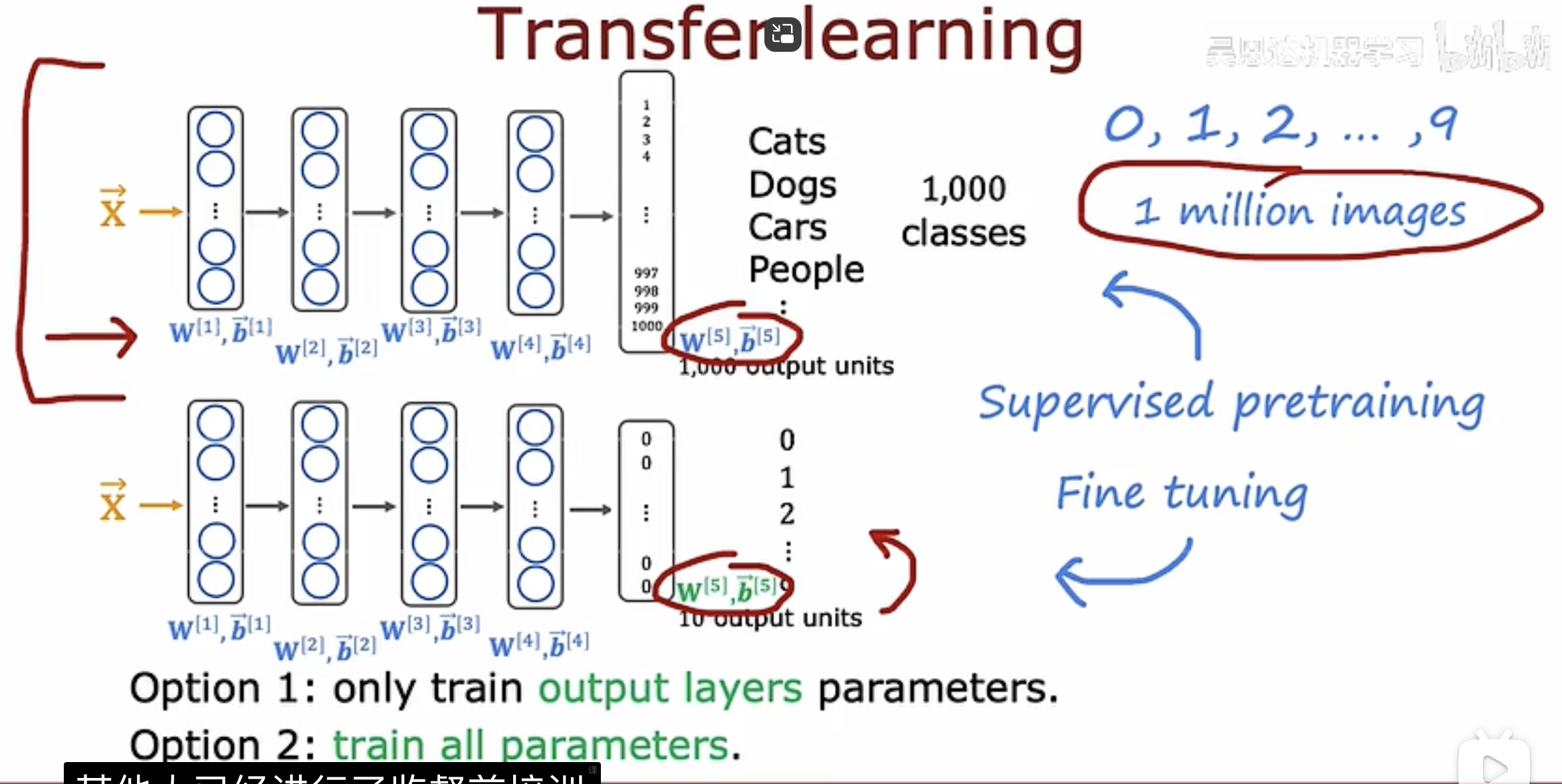
but… why does transfer training work?? I mean, you even can see that a model perform well in recognizing handwriting numbers after fine tuning from a model that is used to recognize animals.

because previous layers may learn to detect edges/corners/basic shapes/curves - numbers have these features too.

but the technique isn’t panacea.

Precision/recall

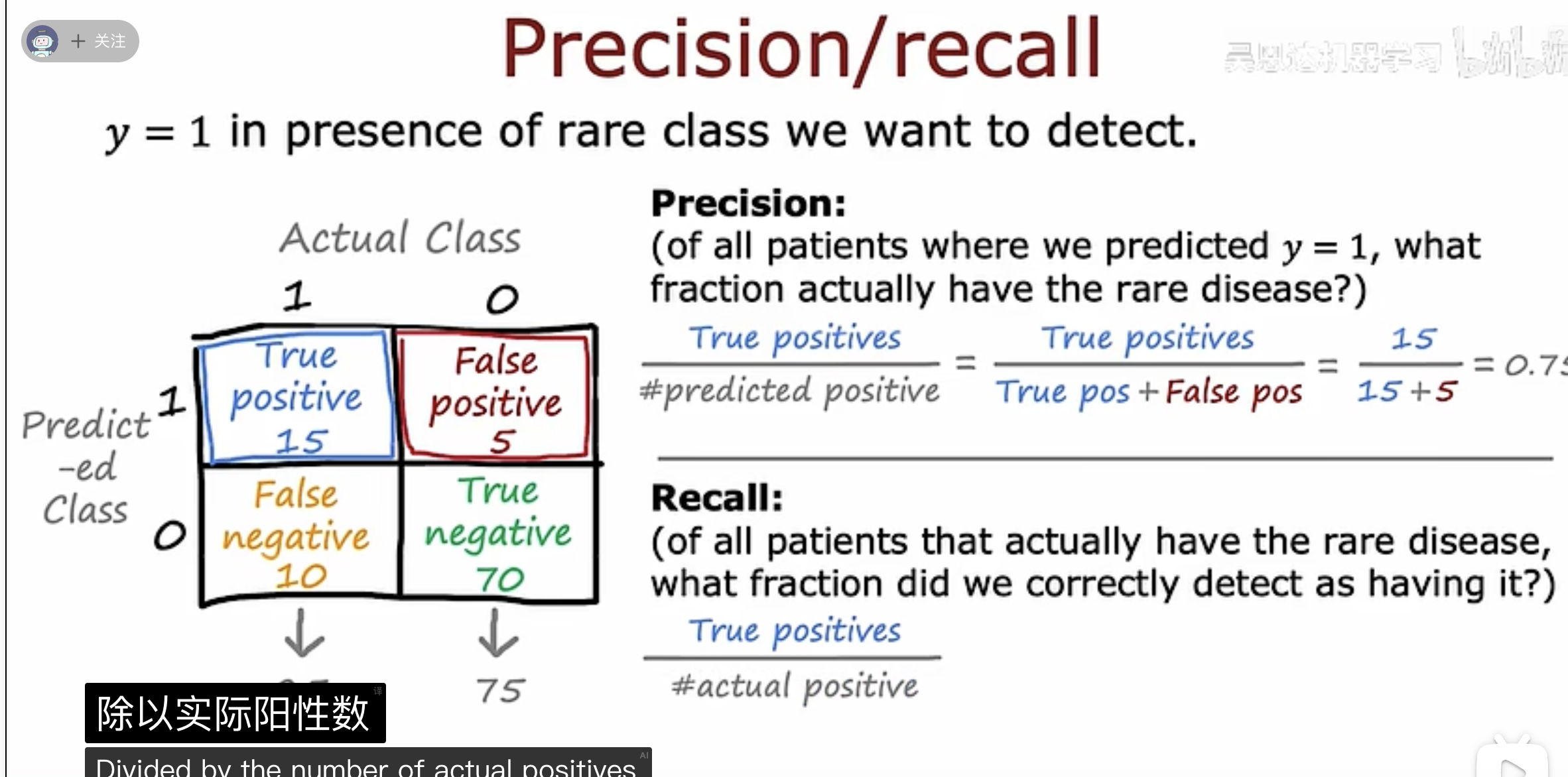
commonly, higher p will lead to lower recall, higher r will lead to lower p.

we can use F1 score to compare p/r numbers.

$F1 score = \frac{1}{\frac{1}{2}(\frac{1}{P} + \frac{1}{R})}$

Convolutional Layer

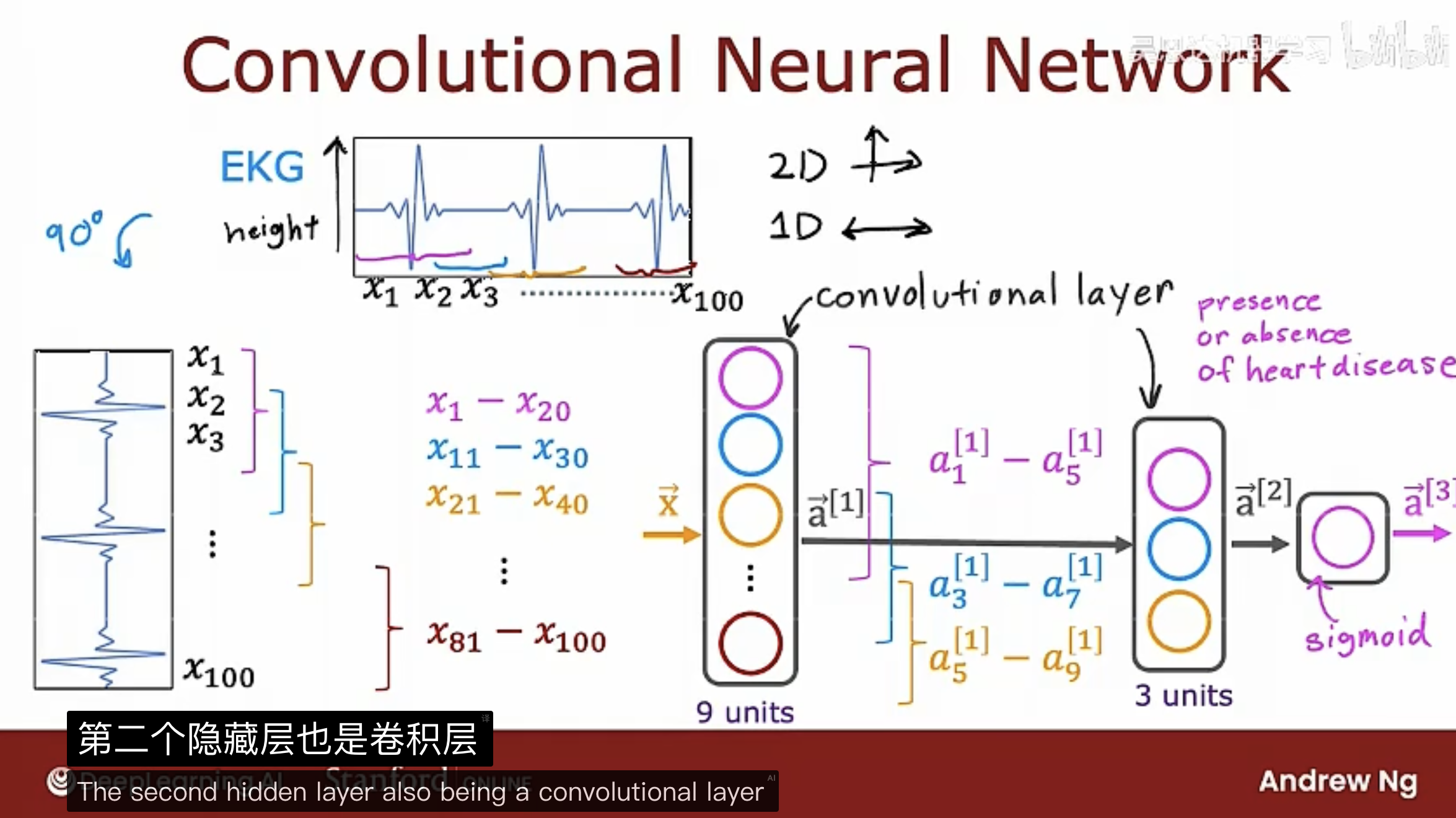
Let each neuron only looks at part of the previous layer’s inputs.

Faster computation.
Need lees training data, less prone to overfitting

Convolutional Neural Network

AKA CNN

Decision Tree

Purity

Information Gain: classification problem

由于一个node有多类多个数据有多个特征，我们需要决定如何去split。

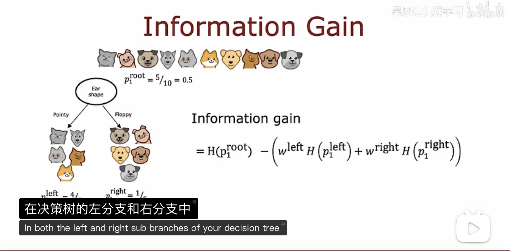
遍历所有的特征，然后计算 information gain。

信息增益的计算方式反映了使用特征 A 进行划分后，节点纯度的提升情况。当信息增益越大时，说明使用特征 A 进行划分后，节点纯度提升得越多，因此选择该特征进行划分可以获得更好的分类效果。

when we splitting on a continuous variable of a feature, we should determine a threshold that split the feature. For example, in a feature called weight we have 10 values, we should test 9 different possible values.

Regression with Decision Tree: Predicting a number

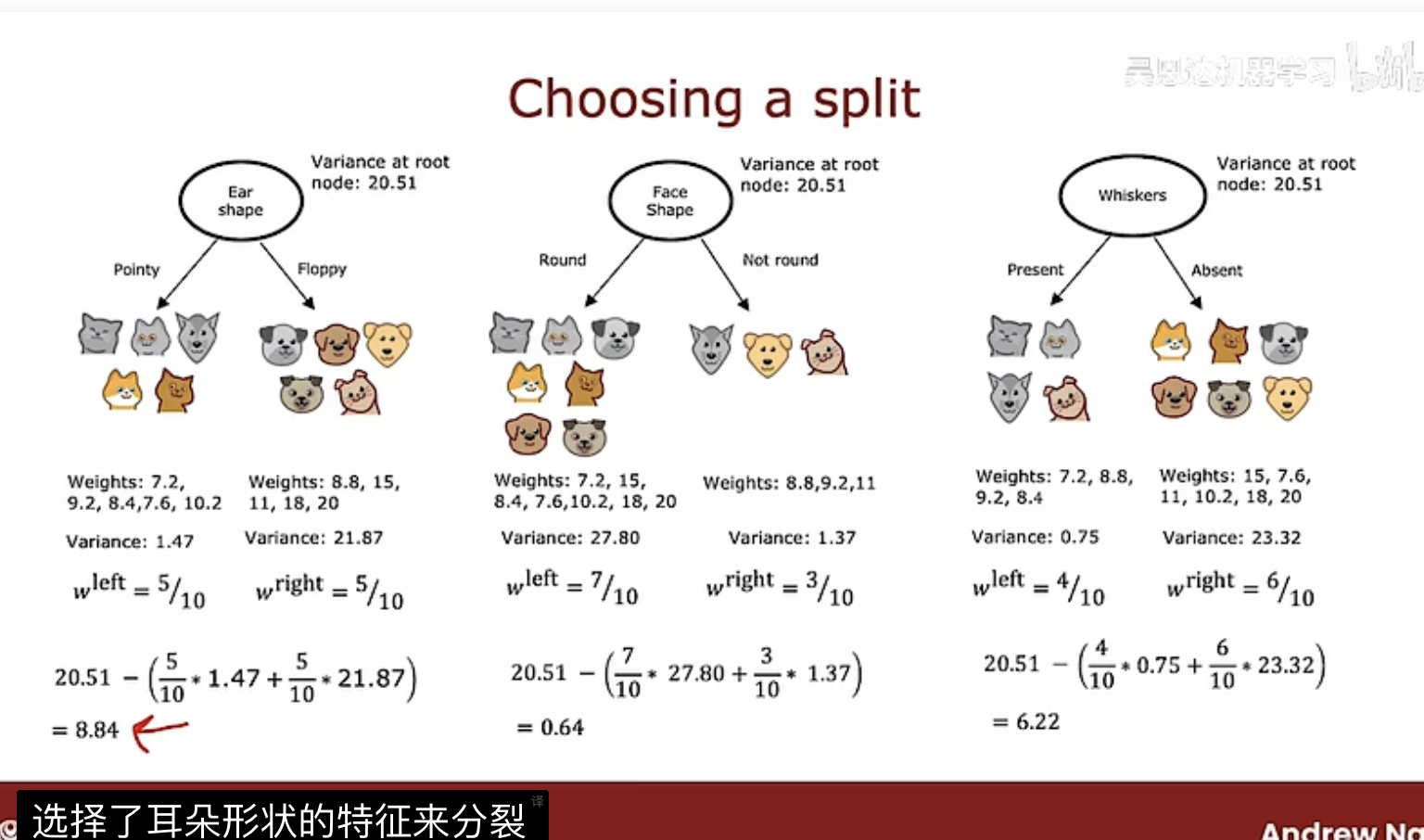
Multiple decision tree

在训练一个决策树的时候，我们往往会选择一个训练例子去构建树。当选择不同的训练例子，得到的树可能会完全不同，这样我们使用这些树进行最终决策就能得到更加准确的结果。

Given training set of size m
For b = 1 to B:
Use sampling with replacement to create a new training set of size m. Train a new tree on the new dataset. When feature number $n$ is large, pick a random subset of k<n features and allow the algorithm to only choose from that subset of features. (Ramdom Forest Algorithm) 这有一个好处。如果不随机选 k<n 个，那么从一般情况上来说，我们随机放回抽样最终得到的不同的决策树的root可能有很多是相同的。典型值是 $k=\sqrt{n}$

Boosted Tree

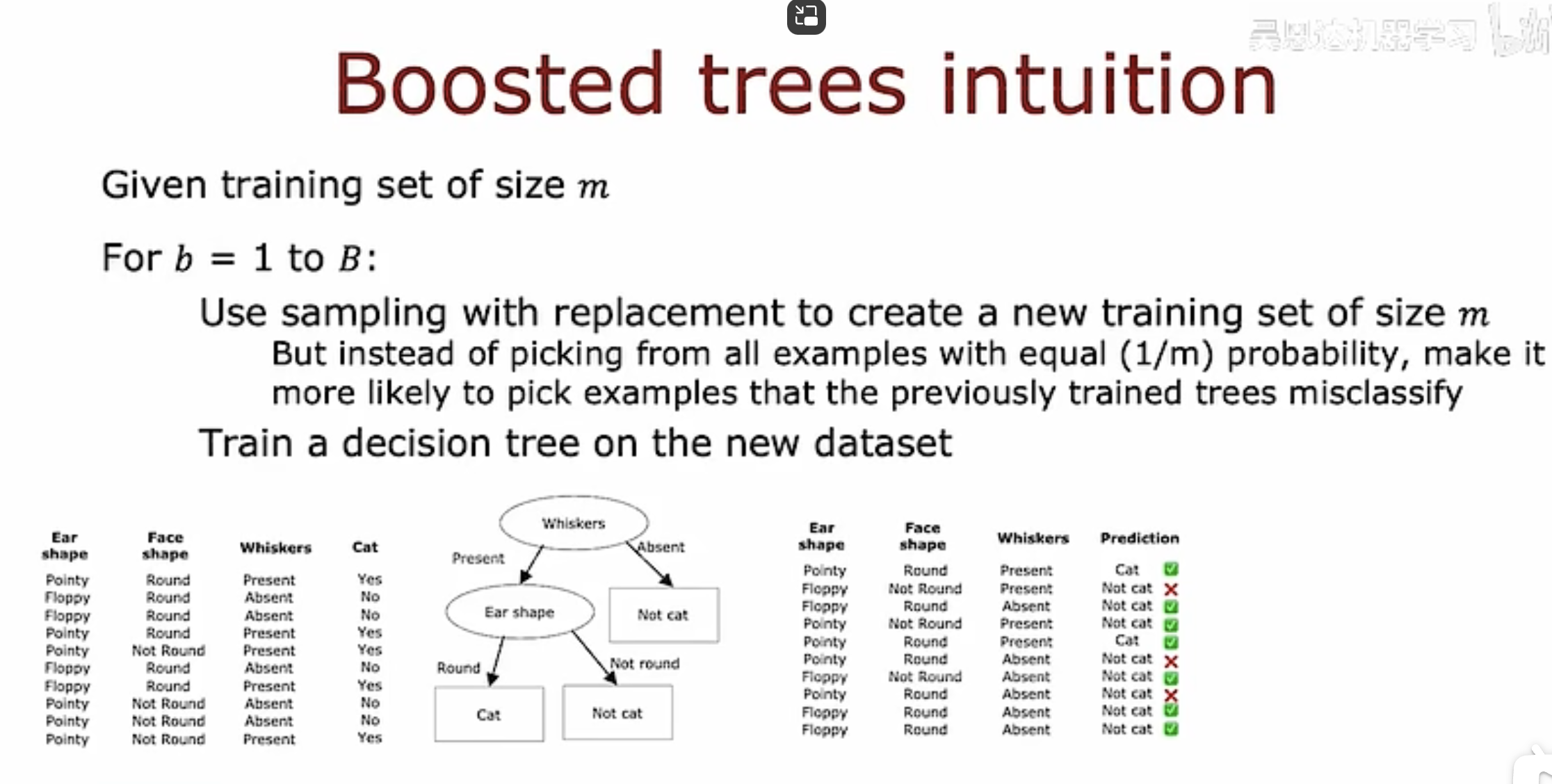
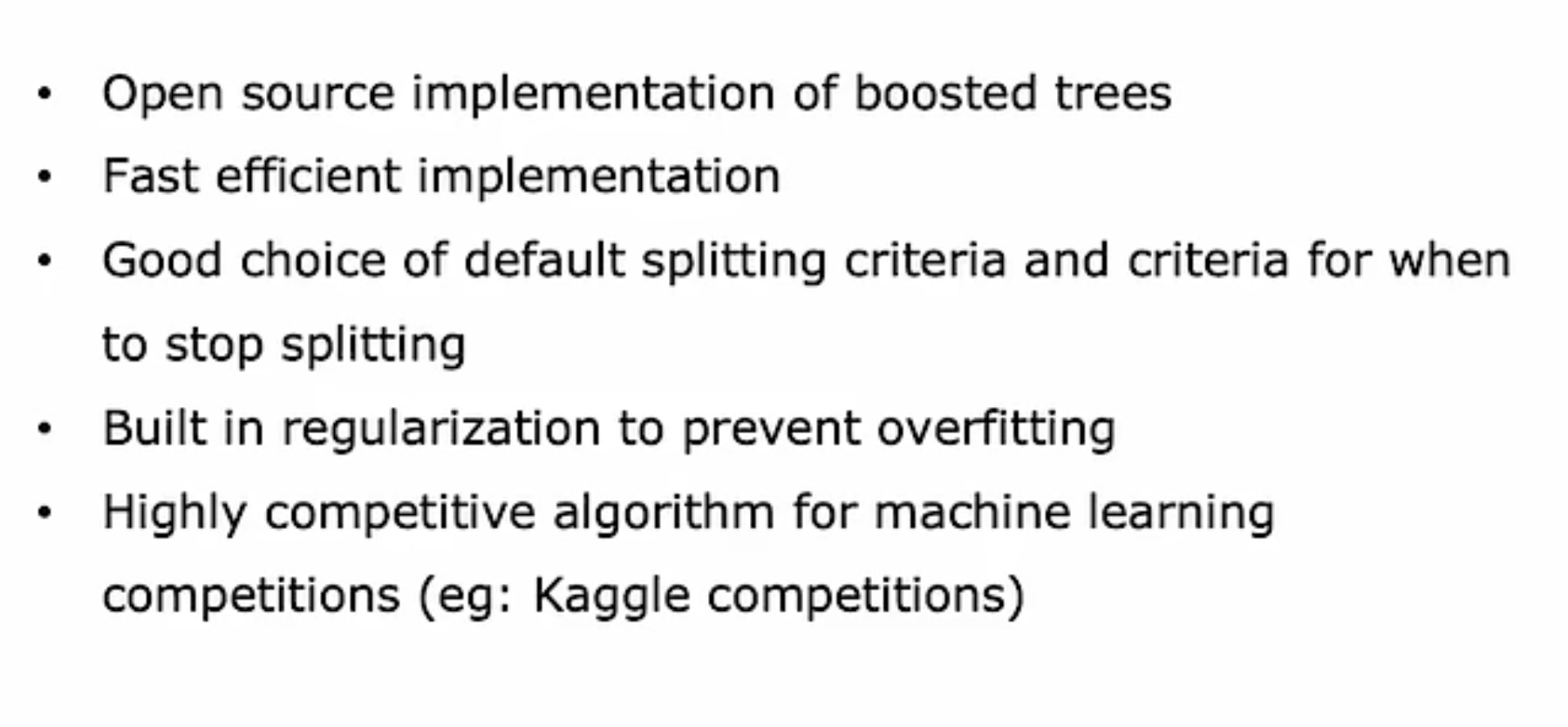
eXtreme Gradient Boosting

When we use DT

Works well on structured data, but not for unstructured data such as images, audio, text.
Fast than NN

NN can works with transfer learning

can easily to string together when you have a system with multiple models.

Unsupervised learning

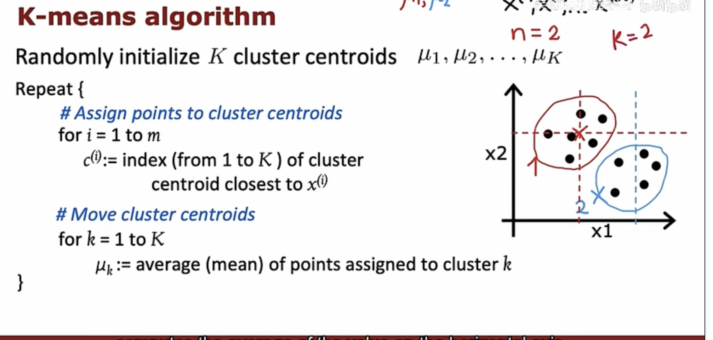
K-means: Clustering Algorithm

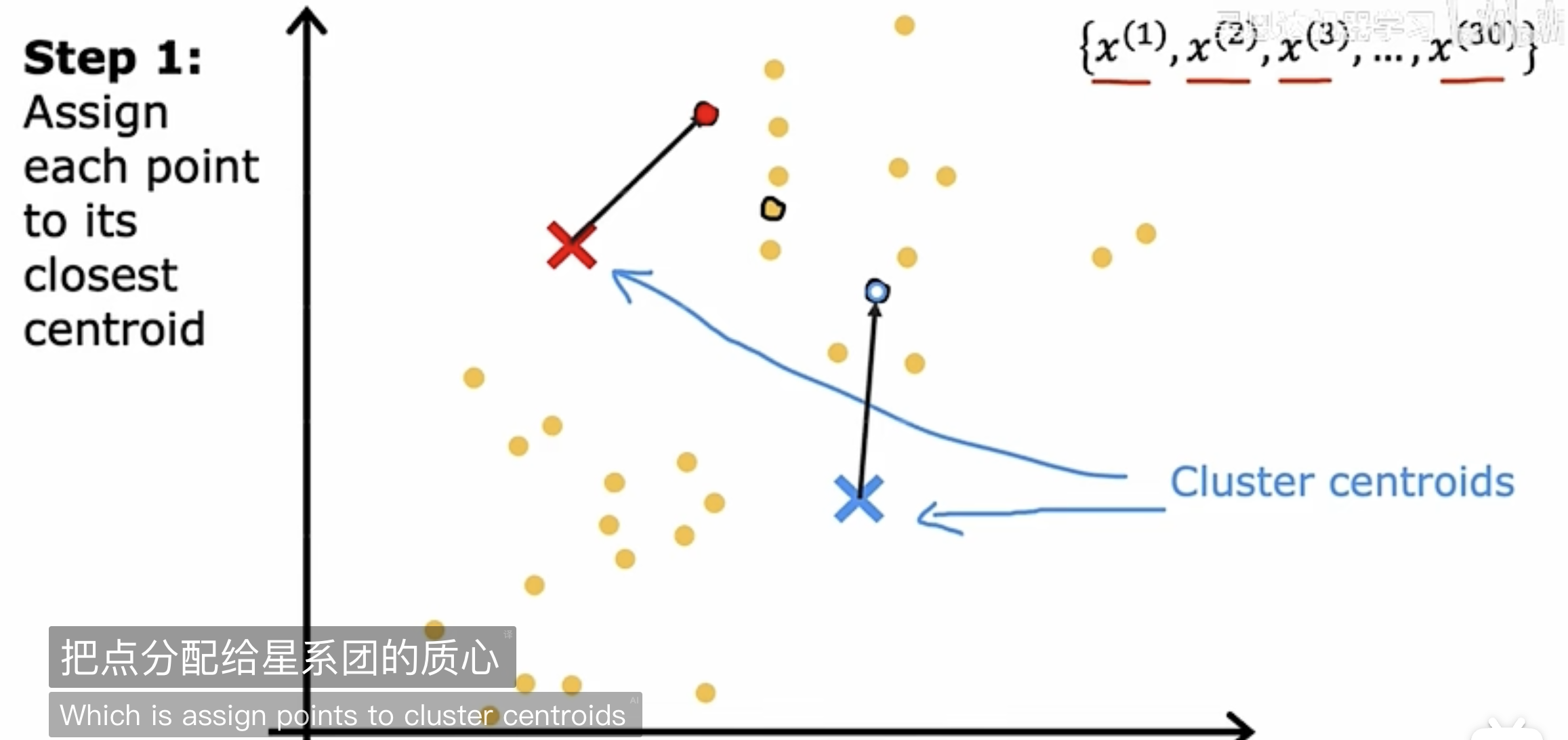
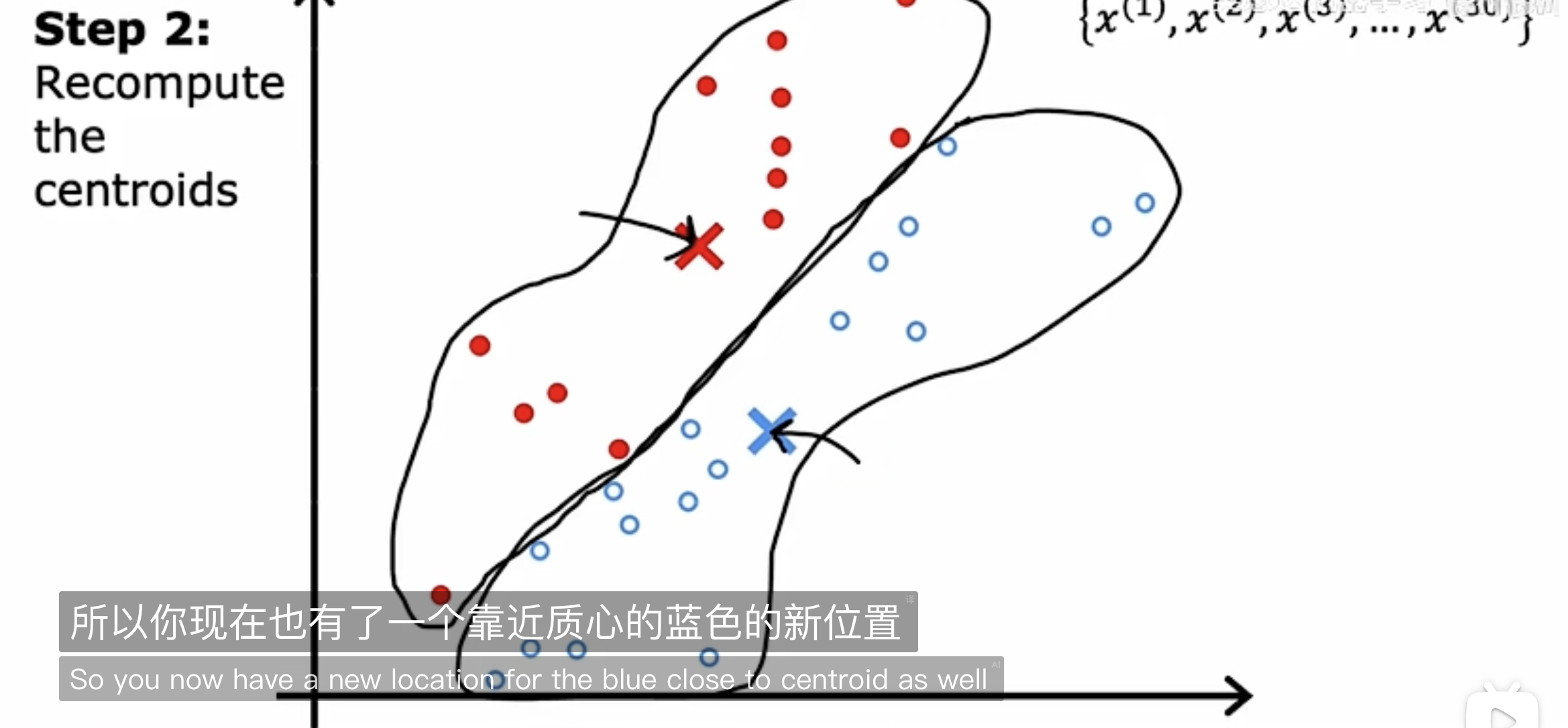
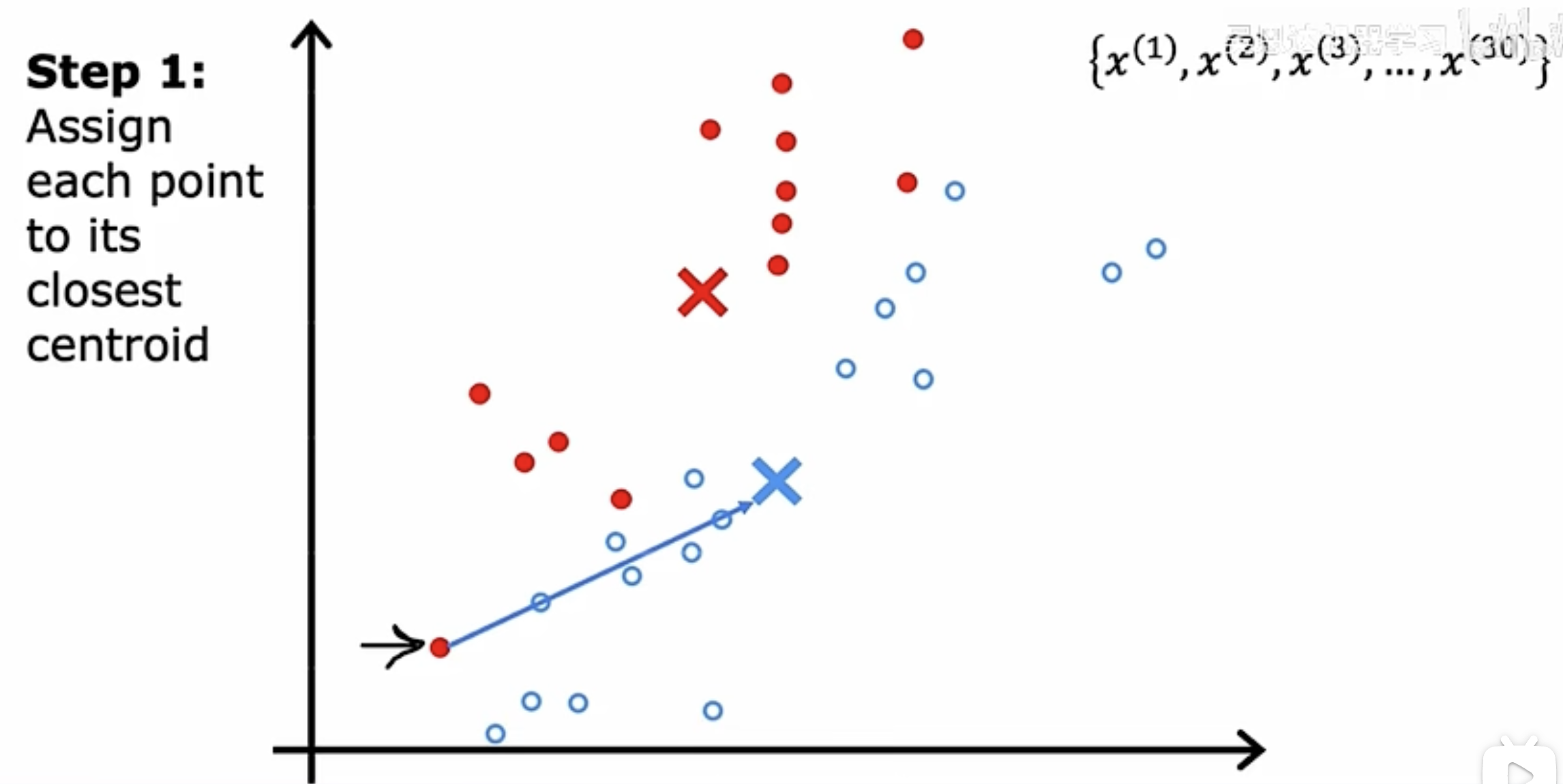
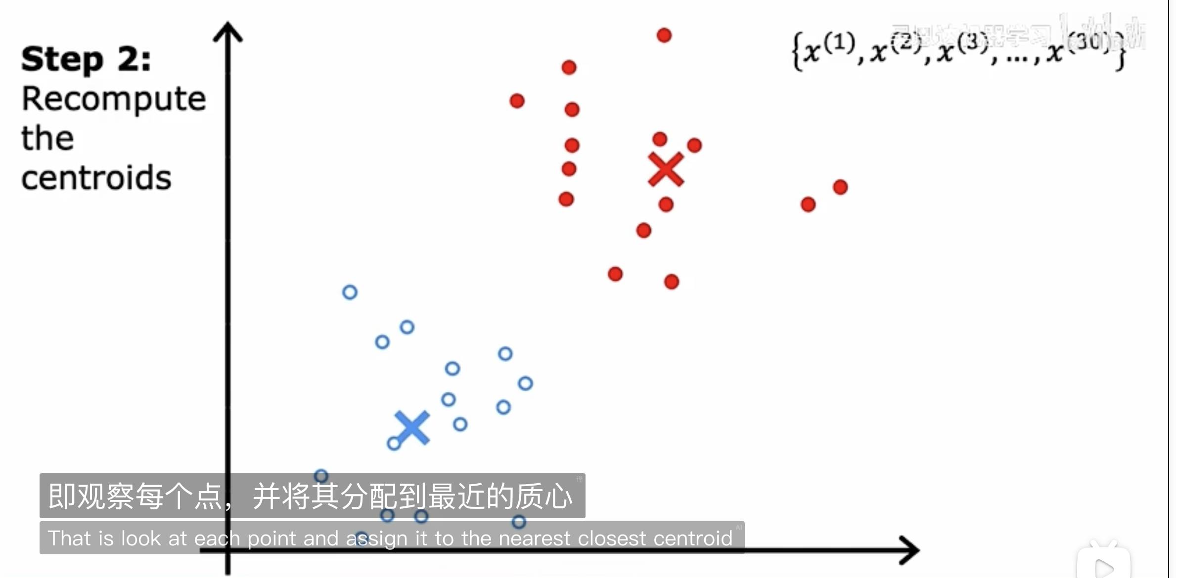
the algorithm

cost function

$J(c^{(1)},...,c^{(m)},\mu_{1},...,\mu_{k}) = \frac{1}{m}\sum_{i=1}^{m}||x^{(i)}-\mu_{c^{(i)}}||^2$

m: the amount of data points

k: amount of clusters

the task k-means algorithm does is minimize the cost. It gotta be converge (why?)

How to initialize k-means better

Choose K<m, randomly pick $K$ training examples. Set $\mu_1,...\mu_k$ equal to these K examples. Might be trapped into the local minumum, so…, we repeat this method for 50-1000 times and select set of clusters that gave the lowest cost J.

How to select the value K

Elbow method:

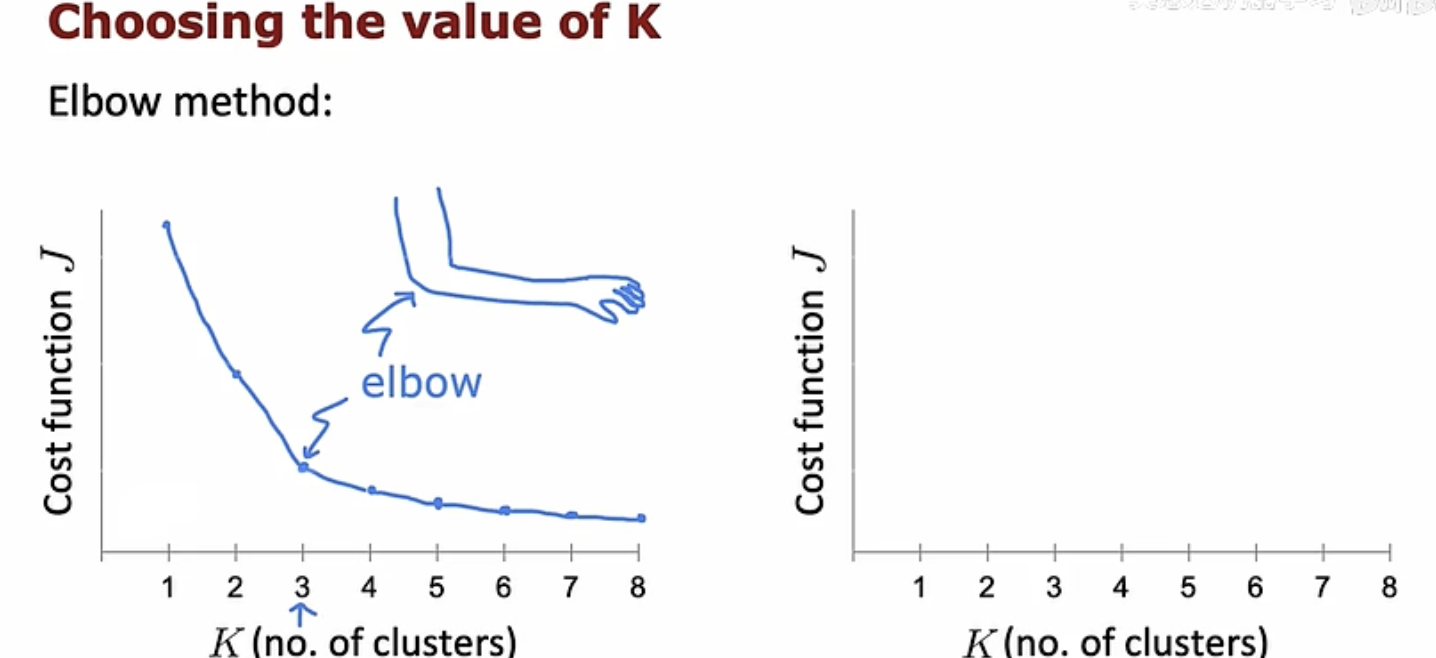
practise

图像压缩（将像素分类到 K 个组中）
各种分类

Anomaly detection

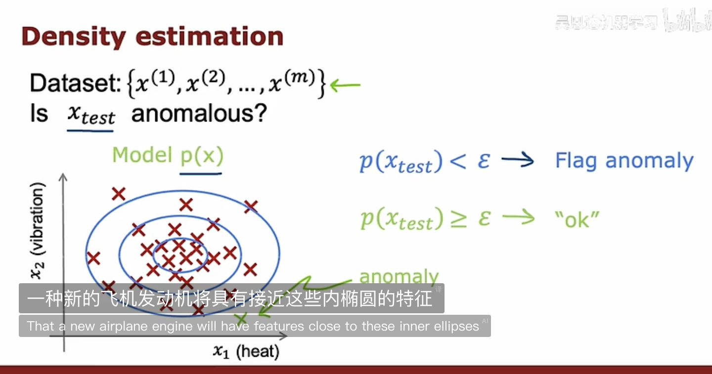
欺诈检测、fake account 检测…

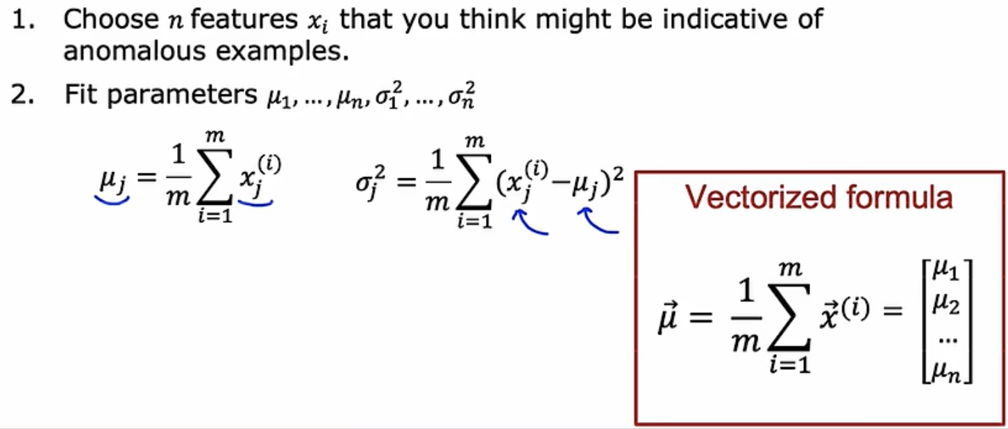
通过划分training set, cv set, test set 去调整 episilon.

Select a epsilon

we use F1-Score to combine precise and recall value.

\begin{aligned} prec&=&\frac{tp}{tp+fp}\\ rec&=&\frac{tp}{tp+fn} \end{aligned}

F_1 = \frac{2\cdot prec \cdot rec}{prec + rec}

epsilon = for eps in range(min(cv_predict_val), max(cv_predict_val), step_size)

def select_threshold(y_val, p_val): 
    """
    Finds the best threshold to use for selecting outliers 
    based on the results from a validation set (p_val) 
    and the ground truth (y_val)
    
    Args:
        y_val (ndarray): Ground truth on validation set
        p_val (ndarray): Results on validation set
        
    Returns:
        epsilon (float): Threshold chosen 
        F1 (float):      F1 score by choosing epsilon as threshold
    """ 

    best_epsilon = 0
    best_F1 = 0
    F1 = 0
    
    step_size = (max(p_val) - min(p_val)) / 1000
    
    for epsilon in np.arange(min(p_val), max(p_val), step_size):
    
        ### START CODE HERE ### 
        predictions = (p_val < epsilon)
        tp = np.sum((predictions == 1) & (y_val == 1))
        fn = np.sum((predictions == 0) & (y_val == 1))
        fp = sum((predictions == 1) & (y_val == 0))
        prec = tp / (tp + fp)
        rec = tp / (tp + fn)
        F1 = 2 * prec * rec / (prec + rec)
        ### END CODE HERE ### 
        
        if F1 > best_F1:
            best_F1 = F1
            best_epsilon = epsilon
        
    return best_epsilon, best_F1

建议

对于非正态分布的特征数据，我们需要 transform it. 比如套一个 $y=log(x)$ 函数(如果这样转换之后，注意在 cv set 和 test set 和未来的预测数据上都要对相同的特征进行转换)
Choose features that might take on unusually large or small values in the event of an anomaly. 我们有时候还可以对特征进行组合。

和监督学习的对比

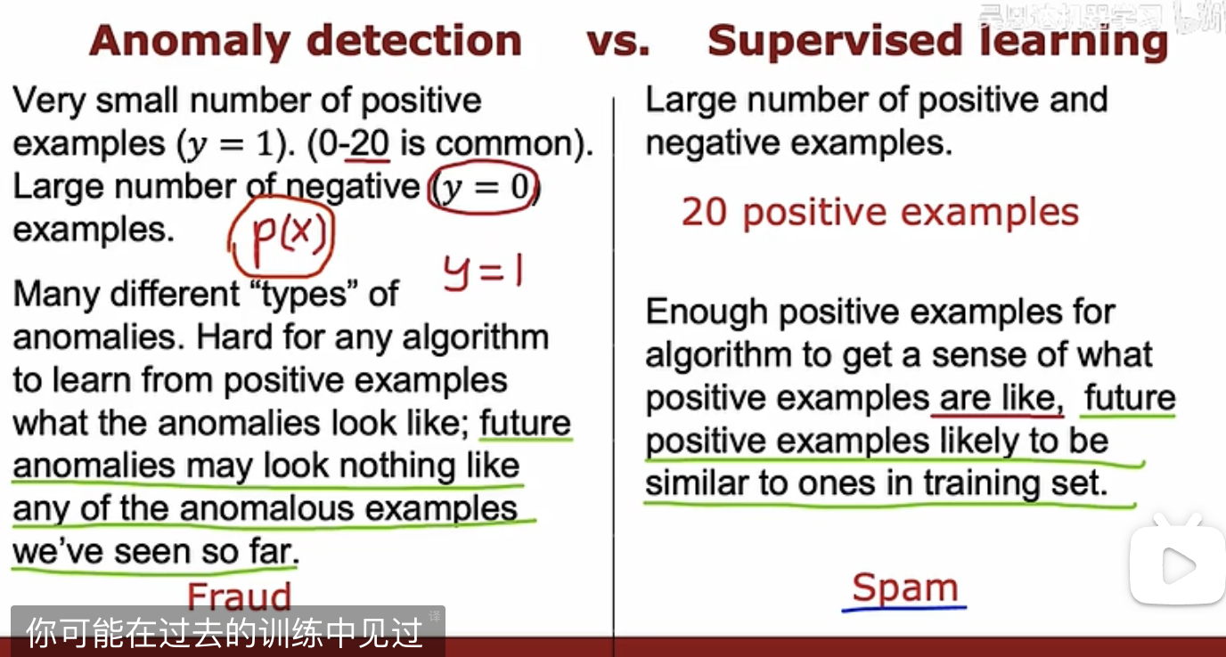
基于训练数据对未来预测数据与自身（模型）的相似性对比。前者是相似度低，后者是相似度高。